Demystifying Deep Learning: Part 8
Convolutional Neural Networks
September 04, 2018
10 min read

Introduction
In this blog post, we’ll look at our first specialised neural network architecture - the convolutional neural network. There is a Jupyter notebook accompanying the blog post containing the code for classifying handwritten digits using a CNN written from scratch.
Motivation for a specialised architecture
Recall in our feedforward neural network post that the weight matrices for layer were stored in a x matrix. Therefore, the number of parameters in the first layer of the network is determined by the number of features in layer 0 (the input layer).
Images are stored in a large multidimensional array of pixels, whose dimensions are (width x height) for greyscale and (width x height x 3) array for RGB images. So consider a small 256x256 RGB image - this results in 256x256x3= 196608 pixels! Each pixel is an input feature, which means that even if we only have 128 units in the first layer, the number of parameters in our weight matrix is 128*196608 = 25 million weights!
Given that most images are much more high-res than 256x256, the number of input features will increase dramatically - for a 1024x1024 RGB image the number of pixels increases by a factor of 16.
This poses a scalability issue - our model has far too many weights! This requires a huge amount of memory and computational power to train. How then do we train a neural network on an image?
Intuition
The key insight is as follows: If we are trying to classify an object in an image, the position of that object in the image does not matter.
So the features we should be learning ought to be independent of position.
This simplifying assumption is at the heart of the convolutional neural network (CNN).
Convolution layer
Interpretation 1: Weight sharing between equivalent neurons
The main difference between the convolution layer and the standard layer we used in a feedforward network is weight sharing.
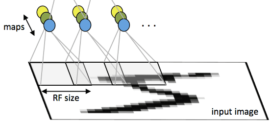
Each neuron in the layer looks at a square patch of the image (the receptive field) - looking at all of the input channels for that image (e.g. RGB channels for the original input image). The neurons take in input from each pixel in that patch and share weights regardless of the position of their patch in the image, so are equivalent.
Interpretation 2: A sliding filter over the image

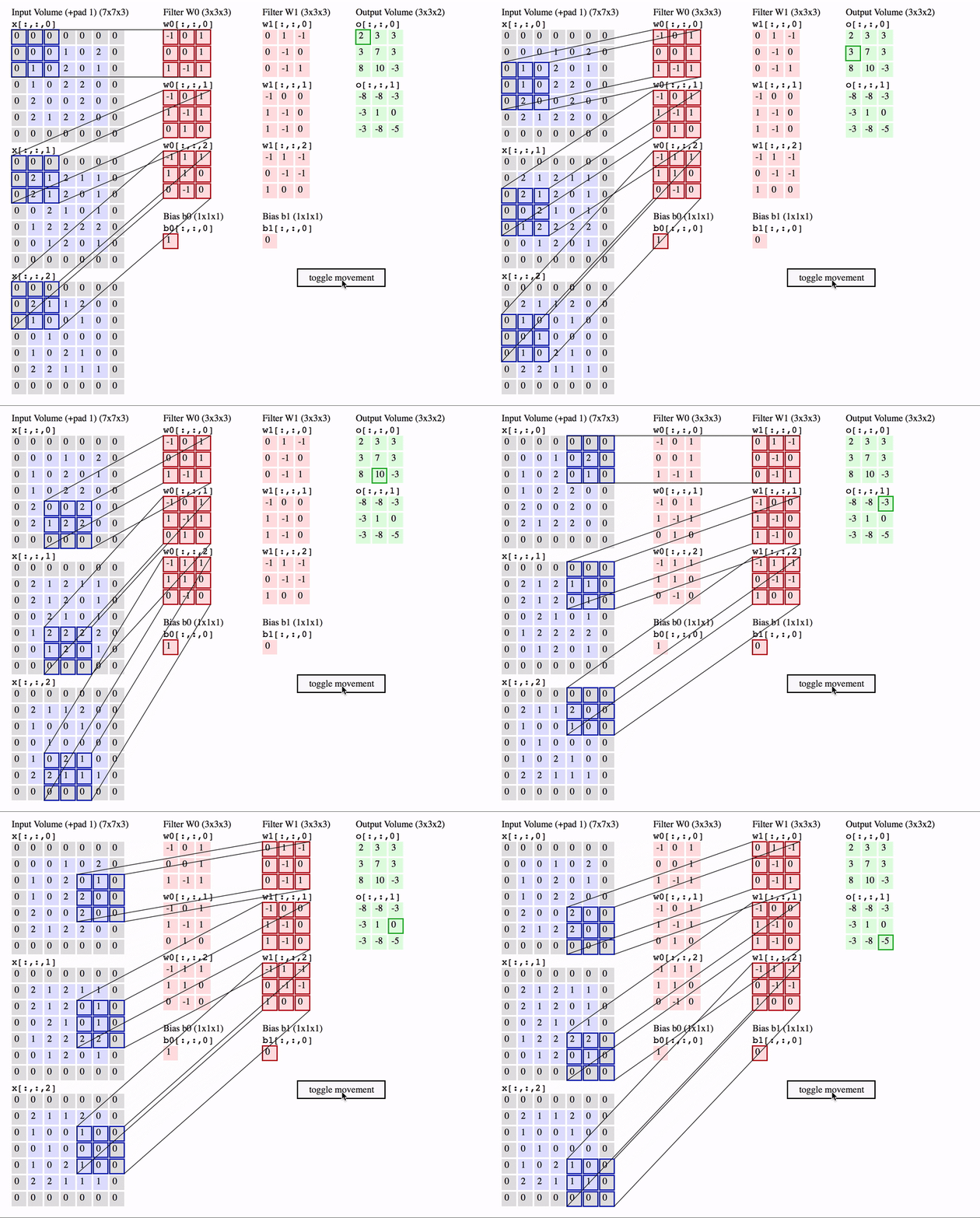
Another interpretation of the convolution layer is, rather than a bunch of equivalent neurons, that of one neuron called the filter / kernel that scans over the image, patch by patch.
Much like the standard neuron we have seen in a feedforward network, the filter weights its inputs (the pixels in that patch) and then applies an activation function to it, to output a single value for that patch.
To compute the weighted input, the filter computes an element-wise product between the pixels in the patch and the corresponding value in its weight matrix - then sums up these to produce an output.
Intuitively, the filter can be seem as a feature detector which produces a high activation when it detects that feature.
So for a single patch starting at position in the image the equation is ( is an element-wise product):
We can take all the activations from each patch across the image to form a 2D feature map / activation map.
The name convolution layer, comes from the mathematical “sliding” convolution operation that we perform to get our output. As an aside, technically the convolution operation flips the weight matrix horizontally and vertically before applying the sliding operation, and is applied to a 2D slice of the image, not to all of the input channels. So the equation for a 2D mathematical convolution is (note not indicating the flipped weights):
Again, this is a case where the deep learning terminology differs slightly from the maths, however for our purposes we will refer to the first (deep learning) equation as a convolution.
Hyperparameters
Now that we have discussed the convolution operation, let’s talk about the nuances and “tuning knobs” at our disposal in a convolution layer.
Number of filters:
First, rather than the one filter, we can have multiple filters, each with their own weights and bias, and then take all the activation maps and stack them in the depth dimension.
We thus store the input and output in a 4D array with dimensions , where is the number of channels/ activation maps.
So the equation for position in the activation map in the convolution layer is:
Note we use here to denote the training example (not using due to clash of notation). We also have a stride of 1 (see the Stride section below).
Filter Size:
We can also alter the size of the receptive field of the neuron. The convention is that the receptive field is square. Typical filter sizes we use are:
- 3x3
- 5x5
- 7x7 (less common - only really was used in early days of CNNs)
- 1x1
1x1 convolutions
The last filter size (1x1) may seem a little surprising. This seems counter-intuitive because there is no spatial information, since you are only looking at one pixel in the image. However, remember we weight and sum across input channels - so we can weight the relative significance each activation map at that point.
The 1x1 convolution is also a cheap way to add depth and non-linearities to the network, since in essence you just have a vector of feature activations and you are doing a matrix multiplication rather like a generalised version of logistic regression across input channels (although using ReLU not sigmoid as the activation function).
1x1 convolutions also have another purpose - depth reduction. Since we stack our feature maps along the depth axis, if we have filters in the previous convolution layer, the depth of the input to this layer will be . If is large, say 256 or 512, then the input becomes rather large. By using fewer filters in this 1x1 convolution layer, the output will have a much smaller depth as a result.
Stride
The stride of the filter is the number of steps the filter slides along between scanning one patch and scanning the next. In nearly all cases, we set a stride of 1 pixel, i.e. scan the next patch. The advantage of having a larger stride is that we can reduce the height/width of the output and thus reduce the size of the output’s dimensions.
However, in practice having a stride of 2 pixels or more is seen as too aggressive and the dimensions reduction is at the expense of a lot of information lost.
For our purposes, when we write equations for the convolution layer, we will assume a stride of 1 pixel.
Padding
Notice how when we scan the image, the pixels in the middle are scanned over multiple times, whereas the pixels at the edge are not scanned over as many times, so we could lose information around the edges of the input.
To ensure we scan these edges an equal number of times as the pixels in the image, we can zero-pad the border of the image - i.e. add a border of zeros around the image. We use zeros to ensure we don’t add any extra information (since the elementwise product over the padded part will be zero).
Let’s calculate the expected output width of the activation map, given an input width and a filter size of . (The calculation for height is identical assuming a square image)
The filter starts off at the left-hand side of the image computing one activation. There are W-1 pixels left to place the top left weight of the filter. However, since the furthest the filter can go is when the right edge of the filter reaches the right edge of the image, this means we cannot place the top left weight in the last pixels. So therefore there are another potential patches to scan.
If we add a padding of pixels to the border of the image, then the effective width is now since we pad each side. So there are patches to scan, excluding the first one it scans.
If we now consider the effect of a stride of pixels, we skip pixels so only scan 1 out of every potential patches. So there are now patches the filter can scan over, excluding the first one it scans.
So the output width: .
This leads us to the values of the hyperparameter . One option is to not have padding at all - we call this setting a valid convolution.
If we look at the complicated expression for the output width, it is hard to keep track of the dimensionality of the input. So, rather than letting the convolution layer reduce the dimensionality, we zero-pad to maintain the dimensionality (set ) - we call this a same convolution.
Code:
ndimage.convolve() takes inputs two n-d arrays and performs an n-dimensional convolution operation on it.
Since we want to perform a 2d convolution, we pass in 2d slices of the input, and sum across the depth of the input. Since in a mathematical convolution, the filter is flipped, we flip the filter beforehand to cancel out the reflection done by ndimage.convolve.
One subtlety is that ndimage.convolve starts convolution from centre of kernel and zero pads but we don’t want this since we want to manually decide if we want to pad or not. So we ignore the edges of the output with a slice [ f//2:-(f//2), f//2:-(f//2) ], where f is the filter size
def conv_forward(x,w,b,padding="same"):f = w.shape[0] #size of filterif padding=="same":pad = (f-1)//2else: #padding is valid - i.e no zero paddingpad =0n = (x.shape[1]-f+2*pad) +1 #ouput width/heighty = np.zeros((x.shape[0],n,n,w.shape[3])) #output array#pad inputx_padded = np.pad(x,((0,0),(pad,pad),(pad,pad),(0,0)),'constant', constant_values = 0)#flip filter to cancel out reflectionw = np.flip(w,0)w = np.flip(w,1)for m_i in range(x.shape[0]): #each of the training examplesfor k in range(w.shape[3]): #each of the filtersfor d in range(x.shape[3]): #each slice of the inputy[m_i,:,:,k]+= ndimage.convolve(x_padded[m_i,:,:,d],w[:,:,d,k])[f//2:-(f//2),f//2:-(f//2)] #sum across depthy = y + b #add bias (this broadcasts across image)return y
ReLU layer
This layer simply takes the convolution layer output and applies the ReLU activation function to it. Having the ReLU operation as a separate layer makes our backpropagation calculations easier, since we can split it into chunks.
We use ReLU because the gradient is either 0 or 1 - if 1 it means the gradient doesn’t diminish as we propagate it through the ReLU. If we were to use sigmoid or tanh, the gradient diminishes (since , the max value of is 0.25). This is the vanishing gradient problem: the gradient gets smaller as we go back through the network and thus the earlier layers’ weights aren’t updated significantly. We’ll look at this problem more in the context of recurrent neural networks later in the series.
In a typical CNN we tend to refer to a convolution layer with the underlying assumption that a ReLU layer follows, rather than explicitly refer to CONV-RELU layers.
Code:
def relu(x, deriv=False):if deriv: #this is for backward passreturn (x>0)return np.multiply(x, x>0) #so this sets x<=0 to 0.
Pooling layer
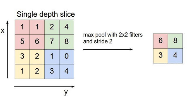
 The pooling layer is another new layer that we use specifically to reduce width/height dimensions - and thus reduce the number of parameters in subsequent layers.
Like the convolution layer, we have a filter, and stride and potential padding, but unlike the convolution layers there are no parameters - instead we apply a function to the patch. NB: unlike in the convolution layer we consider each 2D activation map separately, so we preserve the depth dimension.
The pooling layer intuitively stems from the idea of translational invariance - we don’t care about the precise pixel position of a feature in the patch - it doesn’t matter where in the patch it is so long as it is present somewhere.
With the pooling layer, we almost always set , with no padding- this has the effect of halving the input width and height dimensions.
There are two functions we could apply to the patch in pooling:
- Max-pooling - we take the maximum pixel value for that patch.
- Average-pooling - we average the pixel values in that patch.
In practice we tend to use max-pooling more often than average-pooling as empirically it works better on most computer vision tasks.
Code:
To compute the max/mean of each 2x2 patch we use a neat trick - we reshape the array then take the max/mean along the new axes - this is more efficient that scanning through the image with a for loop. We keep track of the max value in a mask to route gradients through in the backward pass.
def pool_forward(x,mode="max"):x_patches = x.reshape(x.shape[0],x.shape[1]//2, 2,x.shape[2]//2, 2,x.shape[3])if mode=="max":out = x_patches.max(axis=2).max(axis=3)mask =np.isclose(x,np.repeat(np.repeat(out,2,axis=1),2,axis=2)).astype(int)elif mode=="average":out = x_patches.mean(axis=3).mean(axis=4)mask = np.ones_like(x)*0.25return out,mask
Fully-Connected Layer
This is just the standard feedforward neural network layer we have seen. The layer is called fully-connected because each neuron is connected to all the input features. Contrast this with a convolution layer, where (using the equivalent neuron representation) each neuron is only connected to the input pixels in the patch it is looking at.
Again, we typically use ReLU for the fully-connected layers’ activation functions.
Code:
def fc_forward(x,w,b):return relu(w.dot(x)+b)
Softmax Layer
This is a fully-connected layer with the softmax activation function and is the output layer of a neural network for multiclass classification (where we’re predicted if an input is one of multiple classses, not just whether it is a class or not, as in binary classification).
The softmax function is a generalisation of the sigmoid function, in that it too is also assigning a probabilitity to each of the neurons (one neuron for each class).
Given the weighted input of neuron , , the softmax function is as follows:
i.e. we exponentiate the weighted input (think of this as a non-linear scaling), then we divide by the sum of the exponentiated outputs of all the neurons in the layer to normalise the input. This ensures our probabilities sum to 1.
The sigmoid function can be seen as the specific case when we have two units in the output layer - one of which is used for the prediction and the other is a “control” unit with (to normalise the output). So the output for the prediction neuron is:
Code:
def softmax_forward(x,w,b):z = w.dot(x)+bz -= np.max(z,axis=0,keepdims=True) #to prevent overflowa = np.exp(z)a = a/np.sum(a,axis=0,keepdims=True)return a+1e-8 #add 1e-8 to ensure no 0 values - since log 0 is undefined
A typical CNN architecture
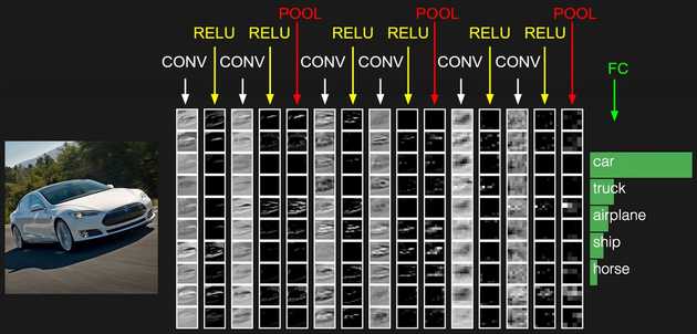
A typical CNN will consist of a few CONV-RELU layers, followed by a POOL layer, and then repeat this a few times, finally having one or two fully-connected layers, followed by the output (softmax) layer. See the above image for an example.
As we go through the network the number of filters typically increases, and like a neural network the features learnt by the filters are hierarchical. The first layer’s filters learn simple features like edges, and subsequent layers build upon this to detect shapes and more complex and abstract objects. We will visualise these in the next blog post.
Since the pooling reduces the width/height and the number of filters increases, we start with a wide, shallow image and end up with a feature vector learnt by the convolution layers that is narrow but deep. We can then flatten this feature vector (so just 1D array) and pass it to the fully-connected layer.
So rather than passing raw pixels to the network as input we’ve in essence constructed a dense encoding of the input instead, which is why intuitively why CNNs vastly outperform feedforward neural networks. The CNN only has (bias) parameters for a convolution layer, rather than the parameters needed for a fully-connected layer.
Conclusion
In this post we’ve looked at the motivation behind a CNN and the different specialist layers found in the CNN.
We can code up the CNN here, and train it on a motivating example - the classification of handwritten digits (MNIST dataset). This dataset is used as a benchmark for computer vision models.
In the next post we will look at the backpropagation algorithm for a convolutional neural network, and also gain some intuition about the internals of a CNN by visualising the activation maps.

